Computing Functions Across a Rolling Window of Time
The following notebook demonstrates use of the RollingWindow network, which is a wrapper around LinearNetwork that sets sys=PadeDelay(theta, order=dimensions) and uses a few extra formulas / tricks. This network allows one to compute nonlinear functions over a finite rolling window of input history. It is most accurate for low-frequency inputs and for low-order nonlinearities. See [1] for details.
[1]:
%pylab inline
import pylab
try:
    import seaborn as sns  # optional; prettier graphs
except ImportError:
    pass

import numpy as np

import nengo
import nengolib
Populating the interactive namespace from numpy and matplotlib
1. Setting up the network
We first create a RollingWindow network with \(\theta=0.1\,s\) corresponding to the size of the window in seconds, and pick some number of LIFRate neurons (2000). The order of the approximation (the dimension of the network’s state ensemble) defaults to 6, since this was found to give the best fit to neural “time cell” data in rodents.
We also need to create an input stimulus. Here, we use a band-limited white noise process since these methods are optimal for low-frequency inputs. Next, connect this to the input node within the rolling window network.
Additionally, we provide this process to the network’s constructor to optimize its evaluation points and encoders (during the build phase) for this particular process. Note that we do not fix the seed of the process in order to prevent overfitting, but we do make the process long enough (10 seconds) for it to generalize. This step is optional, but can dramatically improve the performance. If process=None the input should ideally be modelled, or the eval_points, (orthogonal)
encoders, and radii should be manually specified.
[2]:
process = nengo.processes.WhiteSignal(10.0, high=15, y0=0)
neuron_type = nengo.LIFRate()  # try out LIF() or Direct()

with nengolib.Network() as model:
    rw = nengolib.networks.RollingWindow(
        theta=0.1, n_neurons=2000, process=process, neuron_type=neuron_type)

    stim = nengo.Node(output=process)

    nengo.Connection(stim, rw.input, synapse=None)
/home/arvoelke/anaconda3/envs/py36/lib/python3.6/site-packages/scipy/signal/filter_design.py:1551: BadCoefficients: Badly conditioned filter coefficients (numerator): the results may be meaningless
  "results may be meaningless", BadCoefficients)
2. Decoding functions from the window
Next we use the add_output(...) method to decode functions from the state ensemble. This method takes a t argument specifying the relative time-points of interest, and a function argument that specifies the ideal function to be computed along this window of points. The method returns a node which approximates this function from the window of input history.
The t parameter can either be a single float, or an array of floats in the range \([0, 1]\). The size of t corresponds to the length of the window array \({\bf w}\) passed to your function, and each element of the t array corresponds to the normalized delay in time for its respective point from the window. The function parameter must then accept a parameter w that is sized according to t, and should output the desired function from the given window w. Decoders
will be optimized to approximate this function from the state of the rolling window network.
For example:
add_output(t=0, function=lambda w: w)approximates a communication channel \(f(x(t)) = x(t)\) (Note: this effectively undoes the filtering from the synapse!).add_output(t=1, function=lambda w: w**2)approximates the function \(f(x(t)) = x(t-\theta)^2\).add_output(t=[.5, 1], function=lambda w: w[1] - w[0])approximates the function \(f(x(t)) = x(t-\theta) - x(t-\theta/2)\).
By default, t will be 1000 points spaced evenly between 0 and 1. For example:
add_output(function=np.mean)approximates the mean of this sampled window.add_output(function=np.median)approximates a median filter.add_output(function=np.max)approximates the size of the largest peak.add_output(function=lambda w: np.argmax(w)/float(len(w)))approximates how long ago the largest peak occured.
The function can also return multiple dimensions.
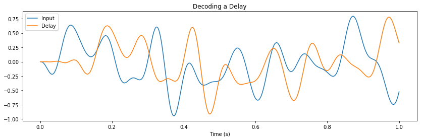
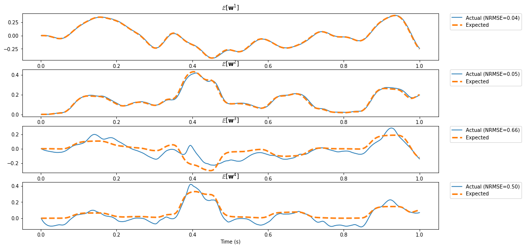
Here we compute two functions from the same state: (1) a delay of \(\theta\) seconds, and (2) the first four moments of the window.
[3]:
with model:
    delay = rw.output  # equivalent to: rw.add_output(t=1)

    def compute_moments(w):
        """Returns the first four moments of the window x."""
        return np.mean(w), np.mean(w**2), np.mean(w**3), np.mean(w**4)

    moments = rw.add_output(function=compute_moments)
3. Set up probes
[4]:
tau_probe = 0.01  # to filter the spikes

with model:
    p_stim_unfiltered = nengo.Probe(stim, synapse=None)

    p_stim = nengo.Probe(stim, synapse=tau_probe)  # filter for consistency

    p_delay = nengo.Probe(delay, synapse=tau_probe)

    p_moments = nengo.Probe(moments, synapse=tau_probe)

    p_x = nengo.Probe(rw.state, synapse=tau_probe)  # for later analysis
4. Simulate the network
[5]:
with nengo.Simulator(model, seed=0) as sim:
    sim.run(1.0)
/home/arvoelke/CTN/nengolib/nengolib/signal/system.py:718: UserWarning: Filtering with non-SISO systems is an experimental feature that may not behave as expected.
  "expected.", UserWarning)
/home/arvoelke/CTN/nengolib/nengolib/signal/system.py:718: UserWarning: Filtering with non-SISO systems is an experimental feature that may not behave as expected.
  "expected.", UserWarning)
5. Plot results
[6]:
# Compute the ideal for comparison
ideal = np.zeros_like(sim.data[p_moments])
w = np.zeros(int(rw.theta / rw.dt))
for i in range(len(ideal)):
    ideal[i] = compute_moments(w)
    w[0] = sim.data[p_stim_unfiltered][i]
    w = nengolib.signal.shift(w)
ideal = nengolib.Lowpass(tau_probe).filt(ideal, dt=rw.dt, axis=0)
[7]:
pylab.figure(figsize=(14, 4))
pylab.title("Decoding a Delay")
pylab.plot(sim.trange(), sim.data[p_stim], label="Input")
pylab.plot(sim.trange(), sim.data[p_delay], label="Delay")
pylab.xlabel("Time (s)")
pylab.legend()
pylab.show()

fig, ax = pylab.subplots(p_moments.size_in, 1, figsize=(15, 8))
for i in range(p_moments.size_in):
    error = nengolib.signal.nrmse(sim.data[p_moments][:, i], target=ideal[:, i])
    ax[i].set_title(r"$\mathbb{E} \left[{\bf w}^%d\right]$" % (i + 1))
    ax[i].plot(sim.trange(), sim.data[p_moments][:, i], label="Actual (NRMSE=%.2f)" % error)
    ax[i].plot(sim.trange(), ideal[:, i], lw=3, linestyle='--', label="Expected")
    ax[i].legend(loc='upper right', bbox_to_anchor=(1.20, 1), borderaxespad=0.)
ax[-1].set_xlabel("Time (s)")
pylab.show()
[8]:
pylab.figure(figsize=(14, 6))
pylab.title("State Space")
pylab.plot(sim.trange(), sim.data[p_x])
pylab.xlabel("Time (s)")
pylab.ylabel(r"${\bf x}$")
pylab.show()
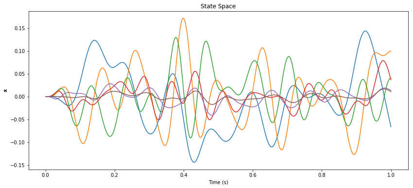
Understanding the network
This network essentially uses the PadeDelay system of order \(d\) to compress the input into a \(d\)-dimensional state \({\bf x}\). This state vector represents a rolling window of input history by a linear combination of \(d\) basis functions:
[9]:
B_canonical = rw.canonical_basis()

pylab.figure()
pylab.title("Canonical Basis")
pylab.plot(nengolib.networks.t_default, B_canonical)
pylab.xlabel("Time (s)")
pylab.show()
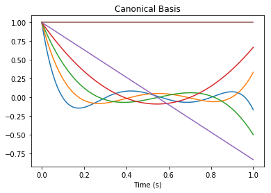
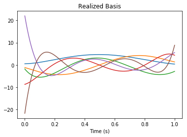
But since the state-space is transformed (by default it is a “balanced realization”), we have the following change of basis (by the linearly independent transformation rw.realizer_result.T):
[10]:
B = rw.basis()
assert np.allclose(B_canonical.dot(rw.realizer_result.T), B)

pylab.figure()
pylab.title("Realized Basis")
pylab.plot(nengolib.networks.t_default, B)
pylab.xlabel("Time (s)")
pylab.show()
Since the encoders of the network are axis-aligned (to improve accuracy of the linear system), this means that the function is able to accurately decode functions of the form:
where \({\bf u}_i\) is the \(i^\texttt{th}\) basis function, \(x_i\) is the corresponding weight given by the state vector \({\bf x}\), and each \(f_i\) is some nonlinear function supported by the neural tuning curves (typically a low-order polynomial).
We now write \({\bf w} = B {\bf x} = \sum_{i=1}^d x_i {\bf u}_i\) where \(B = \left[ {\bf u}_1 \ldots {\bf u}_d \right]\) is our basis matrix, and \({\bf w}\) is the window of history. Then the Moore-Penrose pseudoinverse \(B^+ = (B^T B)^{-1} B^T\) gives us the relationship \({\bf x} = B^+ {\bf w}\), where \(B^+ = \left[ {\bf v}_1 \ldots {\bf v}_d \right]^T\) and ${\bf v}_i $ can be called the \(i^\texttt{th}\) “inverse basis function”. Finally, we can rewrite the computed function \(f\) with respect to the window \({\bf w}\) as:
In other words, the functions that we can compute most accurately will be some linear combination of low-order nonlinearities applied to each \({\bf v}_i \cdot {\bf w}\). Below we visualize each of these inverse basis function:
[11]:
pylab.figure()
pylab.title("Inverse Basis Functions")
pylab.plot(nengolib.networks.t_default, rw.inverse_basis().T)
pylab.xlabel("Time (s)")
pylab.show()

Since the basis functions for the balanced realization are nearly orthogonal, the inverse basis functions are approximately a rescaled version of the former.
Debugging issues in performance
If the desired function is not accurate, then first look at the state-space to see if it is being represented correctly. If not (you might see erratic oscillations or saturation at large values), then there are a few specific things to try:
- Pass a more representative training
process:
- Make sure it corresponds to a typical input stimuli
- Make it aperiodic over a longer time interval (at least 10 seconds)
- Make the process contain higher frequencies (to “activate” all of the dimensions), or decrease the
dimensions, or increasetheta - Make the process contain lower frequencies (to put it within the range of the Padé approximants), or increase the
dimensions, or decreasetheta
- Pass
process=None, and then:
- Set
encodersto be axis-aligned (nengo.dists.Choice(np.vstack([I, -I]))) - Set
radiito the absolute maximum values of each dimension (np.max(np.abs(x), axis=0), after realization) - Set
eval_points=nengolib.stats.cubeor to some representative points in state-space (after radii+realization)
- Change the solver and/or regularization:
- Pass
solver=nengo.solvers.LstsqL2(reg=1e-X)with different X ranging between1and4 - Pass this to either
add_output(to apply only to the decoded function), or to the constructor (to apply to both the recurrent function and the decoded function)
Otherwise, if your function is not expressable as \(\sum_{i=1}^{d} f_i ( {\bf v}_i \cdot {\bf w} )\) for the above \({\bf v}_i\) and for low-order \(f_i\), try:
- Pass a different state-space realization by providing a different
realizerobject to theRollingWindow. SeeLinearNetworkfor details on realizers. This might rotate the state-space into the form of the above (analogous to how the nonlinearProductnetwork is just a diagonal rotation of the linearEnsembleArray). - Create a second ensemble with uniformly distributed encoders (or some other non-orthogonal distribution) and communicate the state variable to that ensemble. Then decode the desired function from that second ensemble using the above basis matrix to define the function with respect to
x. - For expert users, the
RollingWindowis designed to be very “hackable”, in that you can specify many of theEnsembleandConnectionparameters needed to tweak performance, or customize how theprocessis used to solve for theeval_pointsandencoders, or even subclass what happens in_make_core.
References
[1] Aaron R. Voelker and Chris Eliasmith. Improving spiking dynamical networks: accurate delays, higher-order synapses, and time cells. Neural Computation, 30(3):569-609, 03 2018. https://www.mitpressjournals.org/doi/abs/10.1162/neco_a_01046, doi:10.1162/neco_a_01046. [GitHub]

