Geometric Decoder Optimization

This is a way to get an “infinite” number of evaluation points by computing the continuous versions of \(\Gamma = A^T A\) and \(\Upsilon = A^T f(x)\) that we normally use in Nengo. We do so for the scalar case and when \(f(x)\) is a polynomial. The higher dimensional case requires more computational leg-work (Google integrating monomials over convex polytopes).

%pylab inline
import numpy as np
import scipy.linalg
import pylab
try:
    import seaborn as sns  # optional; prettier graphs
    edgecolors = sns.color_palette()[2]
except ImportError:
    edgecolors = 'r'

import nengo
from nengo.neurons import RectifiedLinear, Sigmoid, LIFRate

from nengolib.compat import get_activities

Populating the interactive namespace from numpy and matplotlib

Decoded Function

(Limited to polynomials.)

identity = np.poly1d([1, 0])  # f(x) = 1x + 0
square = np.poly1d([1, 0, 0])  # f(x) = 1x^2 + 0x + 0
quartic = np.poly1d([1, -1, -1, 0, 0])
function = identity

Neuron Model

(Limited to these three for now.)

#neuron_type = RectifiedLinear()
#neuron_type = Sigmoid()
neuron_type = LIFRate()

Baseline Decoders

Let Nengo determine the gains / biases, given: - neuron model - number of neurons - seed

And let Nengo solve for decoders (via MC sampling), given: - function - number of evaluation points - solver and regularization

n_neurons = 10
n_eval_points = 50
solver = nengo.solvers.LstsqL2(reg=0.01)
tuning_seed = None

with nengo.Network() as model:
    x = nengo.Ensemble(
        n_neurons, 1, neuron_type=neuron_type,
        n_eval_points=n_eval_points, seed=tuning_seed)

    conn = nengo.Connection(
        x, nengo.Node(size_in=1),
        function=lambda x: np.polyval(function, x), solver=solver)

with nengo.Simulator(model) as sim: pass

0%

 

eval_points = sim.data[x].eval_points
e = sim.data[x].encoders.squeeze()
gain = sim.data[x].gain
bias = sim.data[x].bias
intercepts = sim.data[x].intercepts

if neuron_type == nengo.neurons.Sigmoid():
    # Hack to fix intercepts:
    # https://github.com/nengo/nengo/issues/1211
    intercepts = -np.ones_like(intercepts)

d_alg = sim.data[conn].weights.T

Refined Decoders

boundaries = e * intercepts
on, off = [], []
for i in range(n_neurons):
    on.append(-1. if e[i] < 0 else boundaries[i])
    off.append(1. if e[i] > 0 else boundaries[i])

Some useful helper functions:

def dint(p, x1, x2):
    """Computes `int_{x1}^{x2} p(x) dx` where `p` is a polynomial."""
    return np.diff(np.polyval(np.polyint(p), [x1, x2]))


def quadratic_taylor(g, dg, ddg):
    """Returns a function that approximates g(ai*ei*x + bi) around x=y."""
    def curve(i, y):
        j = gain[i] * e[i] * y + bias[i]
        f = g(j)
        df = gain[i] * e[i] * dg(j)
        ddf = (gain[i] * e[i])**2 * ddg(j)
        return np.poly1d([
            ddf / 2, df - y * ddf, f - y * df + y**2 * ddf / 2])
    return curve


def segments(x1, x2, max_segments, min_width=0.05):
    """Partitions [x1, x2] into segments (l, m, u) where m = (l + u) / 2."""
    if x1 >= x2:
        return []
    n_segments = max(min(max_segments, int((x2 - x1) / min_width)), 1)
    r = np.zeros((n_segments, 3))
    r[:, 0] = np.arange(n_segments) * (x2 - x1) / n_segments + x1
    r[:, 2] = np.arange(1, n_segments + 1) * (x2 - x1) / n_segments + x1
    r[:, 1] = (r[:, 0] + r[:, 2]) / 2
    return r

Approximate the neuron model using Taylor series polynomials.

if neuron_type == nengo.neurons.RectifiedLinear():
    n_segments = 1
    def curve(i, _):
        return np.poly1d([gain[i] * e[i], bias[i]])

elif neuron_type == nengo.neurons.Sigmoid():
    n_segments = min(n_eval_points, 50)
    ref = x.neuron_type.tau_ref
    g = lambda j: 1. / ref / (1 + np.exp(-j))
    dg = lambda j: np.exp(-j) / ref / (1 + np.exp(-j))**2
    ddg = lambda j: 2*np.exp(-2*j) / ref / (1 + np.exp(-j))**3 - dg(j)
    curve = quadratic_taylor(g, dg, ddg)

elif neuron_type == nengo.neurons.LIFRate():
    n_segments = min(n_eval_points, 50)
    ref = x.neuron_type.tau_ref
    rc = x.neuron_type.tau_rc
    g = lambda j: 1. / (ref + rc * np.log1p(1 / (j - 1)))
    dg = lambda j: g(j)**2 * rc / j / (j - 1)
    ddg = lambda j: (g(j)**3 * rc * (2*rc + ref - 2*j*ref +
                                     (rc - 2*j*rc)*np.log1p(1 / (j - 1))) /
                     j**2 / (j - 1)**2)
    curve = quadratic_taylor(g, dg, ddg)

else:
    raise ValueError("Unsupported neuron type")

Determine a more accurate gamma (G) and upsilon (U) by integrating over the required polynomials. This can be made more efficient.

G = np.zeros((n_neurons, n_neurons))
U = np.zeros(n_neurons)

for i, (li, ui) in enumerate(zip(on, off)):
    for x1, xm, x2 in segments(li, ui, n_segments):
        U[i] += dint(curve(i, xm) * function, x1, x2)
    for j, (lj, uj) in enumerate(zip(on, off)):
        for x1, xm, x2 in segments(max(li, lj), min(ui, uj), n_segments):
            G[i, j] += dint(curve(i, xm) * curve(j, xm), x1, x2)

assert np.allclose(G.T, G)

Invert the gamma matrix and multiply by upsilon, as we normally do:

# d_geo = np.linalg.inv(G).dot(U)

# More complicated decoder solver adapted from:
# https://github.com/nengo/nengo/blob/84db35b5dd673ec715c4b11a0a9afae074f1895f/nengo/utils/least_squares_solvers.py#L32
# in order to make comparisons fair with LstsqL2(reg=reg) where reg > 0.
# Note this is not 'perfect' though because the test set might yield different effective regularization
# than the entire integral. There is probably no way to have a perfect comparison.

# Normalize G and U to be on par with the matrices used by Nengo
# 2 = 1 - (-1) is volume of vector space
G *= len(eval_points) / 2
U *= len(eval_points) / 2

A_nengo = get_activities(sim.model, x, eval_points)
max_rate = np.max(A_nengo)
sigma = solver.reg * max_rate
m = len(eval_points)
np.fill_diagonal(G, G.diagonal() + m * sigma**2)

factor = scipy.linalg.cho_factor(G, overwrite_a=True)
d_geo = scipy.linalg.cho_solve(factor, U)

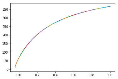
Plot our segmentation of the tuning curve for debugging purposes:

i = 1

x_test = np.linspace(-1, 1, 100000)
x_test = x_test[x_test / e[i] > intercepts[i]]
acts = get_activities(sim.model, x, x_test[:, None])

pylab.figure()
pylab.plot(x_test, acts[:, i], linestyle='--', label="Actual")
for j, (x1, xm, x2) in enumerate(segments(on[i], off[i], n_segments)):
    sl = (x_test > x1) & (x_test < x2)
    pylab.plot(x_test[sl], np.polyval(curve(i, xm), x_test[sl]),
               lw=2, alpha=0.8, label="%d" % j)
pylab.show()

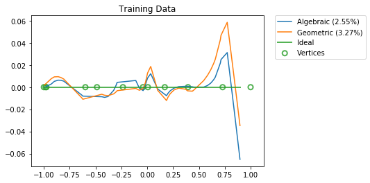
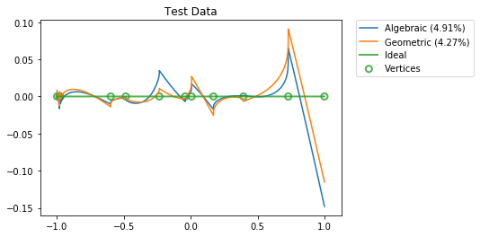
Results

vertices = np.concatenate(([-1], np.sort(boundaries), [1]))

for x_test, title in ((np.sort(eval_points.squeeze()), "Training Data"),
                      (np.linspace(-1, 1, 100000), "Test Data")):
    y = conn.function(x_test)
    activities = get_activities(sim.model, x, x_test[:, None])

    pylab.figure()
    pylab.title(title)
    for d, label in ((d_alg, "Algebraic"),
                     (d_geo, "Geometric")):
        y_hat = np.dot(activities, d).squeeze()
        percent_error = 100 * nengo.utils.numpy.rmse(y_hat, y) / nengo.utils.numpy.rms(y)
        pylab.plot(x_test, y_hat - y, label="%s (%.2f%%)" % (label, percent_error))
    pylab.plot(x_test, np.zeros_like(x_test), lw=2, alpha=0.8, label="Ideal")
    pylab.scatter(vertices, np.zeros_like(vertices), s=50, lw=2, facecolors='none',
                  edgecolors=edgecolors, alpha=0.8, label="Vertices")
    pylab.legend(bbox_to_anchor=(1.05, 1), loc=2, borderaxespad=0.)
    pylab.show()