Linear System Model Reduction

%pylab inline
import numpy as np
import pylab
try:
    import seaborn as sns  # optional; prettier graphs
except ImportError:
    pass

from scipy.linalg import cholesky, svd
from nengo.utils.numpy import rmse

import nengolib
from nengolib import Lowpass

Populating the interactive namespace from numpy and matplotlib

Problem Statement

Suppose we have some linear system. We’d like to reduce its order while maintaining similar characteristics. Take, for example, a lowpass filter that has a small amount of 3rd-order dynamics mixed in, resulting in a 4th-order system that consists mostly of 1st-order dynamics.

isys = Lowpass(0.05)
noise = 0.5*Lowpass(0.2) + 0.25*Lowpass(0.007) - 0.25*Lowpass(0.003)
p = 0.8
sys = p*isys + (1-p)*noise

Exact Minimal Realizations

By cancelling repeated zeros and poles from a system, we can obtain an exact version of that same system with potentially reduced order. However, for the above system, there are no poles to be cancelled, and so this does not help to reduce the order.

assert nengolib.signal.pole_zero_cancel(isys/isys) == 1  # demonstration

minsys = nengolib.signal.pole_zero_cancel(sys)
assert minsys == sys

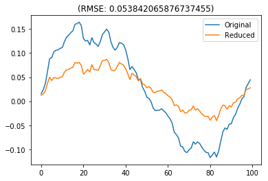
As a crude way of getting around this problem, we can raise the tolerance for detecting similar poles/zeros until repeats are found. By setting the tolerance appropriately for this example, we can reduce the model to a first-order filter, with a surprisingly similar response. However, as we will soon see further down, we can do much better.

minsys_crude = nengolib.signal.pole_zero_cancel(sys, tol=1000.0)
assert minsys_crude.order_den == 1

def test_sys(u, redsys, dt=0.001):
    orig = sys.filt(u, dt)
    red = redsys.filt(u, dt)

    pylab.figure()
    pylab.title("(RMSE: %s)" % rmse(orig, red))
    pylab.plot(orig, label="Original")
    pylab.plot(red, label="Reduced")
    pylab.legend()
    pylab.show()

rng = np.random.RandomState(0)
white = rng.normal(size=100)
test_sys(white, minsys_crude)

Balanced Realizations

First we need to compute some special matrices from Lyapunov theory.

The “controllability gramian” (a.k.a. “reachability gramian” for linear systems) \(W_r\) satisfies:

\[AW_r + W_rA' = -BB'\]

The “observability gramian” \(W_o\) satisfies:

\[A'W_o + W_oA = -C'C\]

See [2] for more background information.

A, B, C, D = sys.ss

R = nengolib.signal.control_gram(sys)
assert np.allclose(np.dot(A, R) + np.dot(R, A.T), -np.dot(B, B.T))

O = nengolib.signal.observe_gram(sys)
assert np.allclose(np.dot(A.T, O) + np.dot(O, A), -np.dot(C.T, C))

The algorithm from [3] computes the lower cholesky factorizations of \(W_r \, ( = L_rL_r')\) and \(W_o \, ( = L_oL_o')\), and the singular value decomposition of \(L_o'L_r\).

LR = cholesky(R, lower=True)
assert np.allclose(R, np.dot(LR, LR.T))

LO = cholesky(O, lower=True)
assert np.allclose(O, np.dot(LO, LO.T))

M = np.dot(LO.T, LR)
U, S, V = svd(M)
assert np.allclose(M, np.dot(U * S, V))

T = np.dot(LR, V.T) * S ** (-1. / 2)
Tinv = (S ** (-1. / 2))[:, None] * np.dot(U.T, LO.T)
assert np.allclose(np.dot(T, Tinv), np.eye(len(T)))

This gives the similarity transform [4] that maps the state to the “balanced realization” of the same order. This system is equivalent up to a change of basis \(T\) in the state-space.

TA, TB, TC, TD = sys.transform(T, Tinv=Tinv).ss
assert sys == (TA, TB, TC, TD)

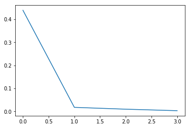
And the reason we do this is because the singular values reflect a measure of importance for each of the states in the new realization. The order should then be reduced by removing the least important states.

pylab.figure()
pylab.plot(S)
pylab.show()

The short-cut to do the above procedure in nengolib is the function balanced_transformation followed by sys.transform:

T, Tinv, S_check = nengolib.signal.balanced_transformation(sys)
sys_check = sys.transform(T, Tinv)

assert np.allclose(TA, sys_check.A)
assert np.allclose(TB, sys_check.B)
assert np.allclose(TC, sys_check.C)
assert np.allclose(TD, sys_check.D)
assert np.allclose(S, S_check)

Lastly, note that this diagonalizes the two gramiam matrices:

P = nengolib.signal.control_gram((TA, TB, TC, TD))
Q = nengolib.signal.observe_gram((TA, TB, TC, TD))

diag = np.diag_indices(len(P))
offdiag = np.ones_like(P, dtype=bool)
offdiag[diag] = False
offdiag = np.where(offdiag)

assert np.allclose(P[diag], S)
assert np.allclose(P[offdiag], 0)
assert np.allclose(Q[diag], S)
assert np.allclose(Q[offdiag], 0)

Approximate Model Order Reduction

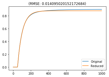
Low singular values indicate states are less important. The method in [5] can be used to remove these states while matching the DC gain for continuous or discrete systems.

redsys = nengolib.signal.modred((TA, TB, TC, TD), 0, method='dc')
assert redsys.order_den == 1

step = np.zeros(1000)
step[50:] = 1.0
test_sys(step, redsys)
test_sys(white, redsys)

/home/arvoelke/CTN/nengolib/nengolib/signal/system.py:214: UserWarning: Synapse ((A=[[0.98382223]], B=[[-0.00375194]], C=[[-3.7826243]], D=[[0.02273466]], analog=False)) has extra delay due to passthrough (https://github.com/nengo/nengo/issues/938).
  "(https://github.com/nengo/nengo/issues/938)." % sys)

/home/arvoelke/CTN/nengolib/nengolib/signal/system.py:214: UserWarning: Synapse ((A=[[0.98382223]], B=[[-0.00375194]], C=[[-3.7826243]], D=[[0.02273466]], analog=False)) has extra delay due to passthrough (https://github.com/nengo/nengo/issues/938).
  "(https://github.com/nengo/nengo/issues/938)." % sys)

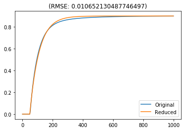
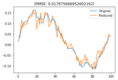
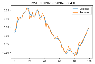
However, this doesn’t work very well for matching the response of the system given white-noise input. If we care less about the steady-state response, then it is much more accurate to simply delete the less important states.

delsys = nengolib.signal.modred((TA, TB, TC, TD), 0, method='del')
assert delsys.order_den == 1
test_sys(step, delsys)
test_sys(white, delsys)

The short-cut for all of the above is to call nengolib.signal.balred with a desired order and method.

References

[1] http://www.mathworks.com/help/control/ref/minreal.html

[2] https://en.wikibooks.org/wiki/Control_Systems/Controllability_and_Observability

[3] Laub, A.J., M.T. Heath, C.C. Paige, and R.C. Ward, “Computation of System Balancing Transformations and Other Applications of Simultaneous Diagonalization Algorithms,” IEEE® Trans. Automatic Control, AC-32 (1987), pp. 115-122.

[4] http://www.mathworks.com/help/control/ref/balreal.html

[5] http://www.mathworks.com/help/control/ref/modred.html