Sampling High-Dimensional Vectors

Aaron R. Voelker (January 15, 2016)

%pylab inline
import numpy as np
import pylab
try:
    import seaborn as sns  # optional; prettier graphs
except ImportError:
    sns = None

import nengo
from nengolib.compat import get_activities
from nengolib.stats import ScatteredHypersphere, Sobol

uniform_ball = nengo.dists.UniformHypersphere(surface=False)
uniform_sphere = nengo.dists.UniformHypersphere(surface=True)

# base=Rd() is now the default
scatter_ball = ScatteredHypersphere(surface=False, base=Sobol())
scatter_sphere = ScatteredHypersphere(surface=True, base=Sobol())

Populating the interactive namespace from numpy and matplotlib

Abstract

The Monte Carlo (MC) method of sampling is notoriously bad at reproducing the same statistics as the distribution being sampled.

def plot_dist(dist, title, num_samples=500):
    pylab.figure(figsize=(4, 4))
    pylab.title(title)
    pylab.scatter(*dist.sample(num_samples, 2).T, s=10, alpha=0.7)
    pylab.xlim(-1, 1)
    pylab.ylim(-1, 1)
    pylab.show()

plot_dist(uniform_ball, 'Uniform 2-Ball')

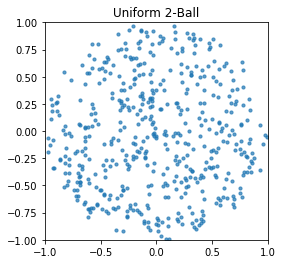
Intuitively, MC sampling gives lots of “gaps” and “clumps”, while instead what we want is more of a “scattering” of points uniformly about the sphere.

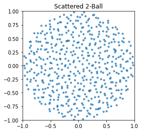
plot_dist(scatter_ball, 'Scattered 2-Ball')

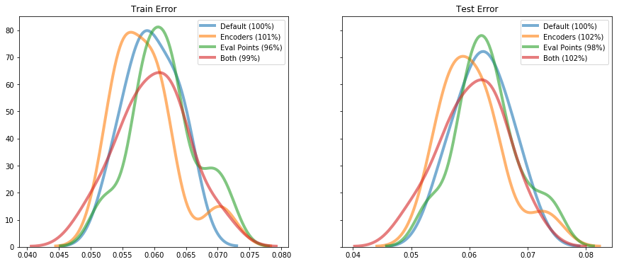
We currently have three reasons to sample vectors in Nengo: 1. Choosing the encoders for a population 2. Choosing the evaluation points to solve for decoders 3. Choosing the semantic pointers in a vocabulary

MC is bad for problem 1, because the neurons should be uniformly representing all parts of the vector space. MC sampling is also bad for problem 2, because the “empirical distribution” does not match the actual distribution unless there are a large number of samples, and so the decoders are biased to minimize the approximation error of certain vectors over others. A scattered distribution overcomes this problem by giving a closer match to the uniform distribution with fewer samples.

In fact, problems 1 and 2 are basically equivalent. When sampling encoders, we are effectively choosing which vectors should have the least error (by principle (1) they fire the most, and then by principle (2) they contribute the most to the estimate). The only ‘real’ difference is that encoders are on the \(D\)-sphere, while evaluation points are on the \(D\)-ball. These two problems can be solved efficiently by the number-theoretic method (NTM), also known as the quasi Monte Carlo method, to generate scattered points. These solutions can then be used to sample encoders and evaluation points, to improve the representation of a population and its decoders.

def do_trial(seed, encoders, eval_points, n_eval_points, test_points, n_test_points,
             n_neurons, dims):
    with nengo.Network(seed=seed) as model:
        # Make a single ensemble and connection
        ens = nengo.Ensemble(
            n_neurons, dims, encoders=encoders, eval_points=eval_points,
            n_eval_points=n_eval_points)
        conn = nengo.Connection(ens, nengo.Node(size_in=dims))

        # Build the model
        built = nengo.builder.Model(decoder_cache=nengo.cache.NoDecoderCache())
        built.build(model)
        with nengo.Simulator(None, model=built, progress_bar=False) as sim:
            pass

        # Find the optimal decoders and their corresponding RMSE on the eval_points
        decoders = sim.data[conn].weights
        eval_rmses = np.mean(sim.data[conn].solver_info['rmses'])

        # Sample some new test_points and test them on the same decoders
        x = test_points.sample(n_test_points, dims, rng=np.random.RandomState(seed))
        a = get_activities(sim.model, ens, x)
        x_hat = np.dot(a, decoders.T)
        test_rmses = nengo.utils.numpy.rmse(x, x_hat, axis=1)

        # Return the average training and test errors
        return np.mean(eval_rmses), np.mean(test_rmses)

def do_experiment(n_neurons, dims, n_eval_points=500, test_points=uniform_ball,
                  n_test_points=500, trials=10):
    fig, ax = pylab.subplots(1, 2, sharey=True, figsize=(15, 6))
    ax[0].set_title('Train Error')
    ax[1].set_title('Test Error')
    default_means = None
    for i, (label, encoders, eval_points) in enumerate((
            ('Default',     uniform_sphere, uniform_ball),
            ('Encoders',    scatter_sphere, uniform_ball),
            ('Eval Points', uniform_sphere, scatter_ball),
            ('Both',        scatter_sphere, scatter_ball))):
        errors = np.empty((trials, 2))
        for seed in range(trials):
            errors[seed] = do_trial(
                seed, encoders, eval_points, n_eval_points,
                test_points, n_test_points, n_neurons, dims)
        means = np.mean(errors, axis=0)
        if default_means is None:
            default_means = means
        for j in range(2):
            l = '%s (%d%%)' % (label, default_means[j] / means[j] * 100)
            if sns is None:
                ax[j].hist(errors[:, j], label=l, lw=1, alpha=0.3)
            else:
                sns.kdeplot(errors[:, j], ax=ax[j], label=l, lw=4, alpha=0.6)
    ax[0].legend()
    ax[1].legend()
    pylab.show()

do_experiment(n_neurons=100, dims=16)

/home/arvoelke/anaconda3/envs/py36/lib/python3.6/site-packages/scipy/stats/stats.py:1713: FutureWarning: Using a non-tuple sequence for multidimensional indexing is deprecated; use `arr[tuple(seq)]` instead of `arr[seq]`. In the future this will be interpreted as an array index, `arr[np.array(seq)]`, which will result either in an error or a different result.
  return np.add.reduce(sorted[indexer] * weights, axis=axis) / sumval

However, problem 3 is strictly harder (and in fact almost completely different), and so we will save that talk for a later day.

The Number-Theoretic Method (NTM)

This exact same problem showed up as early as 1961 and was studied extensively in the 1980s [1] for applications in experimental design and statistical finance, in which the task boils down to evaluating a high-dimensional integral:

\[\int_{S} f({\bf u})\,{\rm d}{\bf u}\]

where \(S\) is some \(D\)-dimensional space. Due to the curse of dimensionality, even modestly sized \(D\) requires too many points to evaluate using standard numerical integration techniques like the trapezoidal rule. Instead, the standard approach is to choose a sub-sampling of representative points \(\{{\bf x_1}, \ldots, {\bf x_N}\}\) over the domain of \(S\), and compute:

\[\approx \frac{1}{N}\,\sum_{i=1}^N f({\bf x_i})\]

This works well as long as we can sample these points uniformly. It has been theoretically proven that the approximation error from using the NTM is superior to that of MC sampling.

---

To make the connection back to our original problem explicit, when solving for the decoders we are minimizing the mean squared error given by:

\[\int_{S} ({\bf x} - {\bf \hat{x}})^2 \,{\rm d}{\bf x}\]

where \(S\) is the \(D\)-ball. Thus, \(f({\bf u}) = ({\bf u} - {\bf \hat{u}})^2\) is the function we need to integrate. And the points \(\{{\bf x_1}, \ldots, {\bf x_N}\}\) are precisely the set of \(N\) evaluation points that we are, in effect, choosing to approximate this integral. This explains more formally why this new approach out-performs the old approach.

---

Now the NTM goes by a number of roughly equivalent names: - uniform design - NT-net - quasi Monte Carlo - quasi-random - low-discrepancy sequence - representative points - uniformly scattered points

We will refer to the collective theory as the NTM, and to a specific sampling as a uniform scattering.

There are many algorithms to generate scattered points in the literature: - Faure - Good Points - Good Lattice Points - [STRIKEOUT:Latin Square] - Haber - Halton (van der Corput) - Hammersley - Hua and Wang (cyclotomic field) - Niederreiter - [STRIKEOUT:Poisson Disk] - Sobol

Since Sobol had the most readily-available Python library (and the largest Wikipedia page), I used it for all my experiments. The default method has been updated to Rd since the writing of this notebook.

All of these approaches (except the Latin Square and Poisson Disk sampling) attempt to minimize the discrepancy of the samples. Informally, the discrepancy measure tells us how much the sample distribution differs from the underlying distribution. Formally, we define the empirical distribution as the cumulative distribution function (CDF) \(F_N({\bf x}) = P({\bf X} \le {\bf x})\), where:

\[P({\bf X} = {\bf x_i}) = \frac{1}{N}, \quad i = 1 \ldots N\]

Then the discrepancy of this set is defined as:

\[D(N) = sup_{x \in \mathbb{R}^D} |F_N({\bf x}) - F({\bf x})|\]

where \(F\) is the true CDF. This gives an upper-bound on how well the empirical CDF approximates the true CDF. The lower this is, the better our sample set represents the true distribution at all points (not just the points that were sampled). And all of these approaches (again, except for Latin/Poisson) have worst-case (guaranteed) bounds that are asymptotically dominated by MC in theory (and for lower \(N\) as well in practice).

\[\begin{split}D(N) = \begin{cases} O(\frac{1}{\sqrt{N}}) & \text{MC Sampling} \\ O(\frac{(log N)^D}{N}) & \text{NTM Sampling} \end{cases}\end{split}\]

The \(\sqrt{N} = o(N)\) is the important part. The numerator is a worst-case that is reported to be a small constant in practice.

The nice fact that comes out of all of this, is that: the discrepancy is related to the error when computing the above integral by a constant factor (fixed for a given \(f\)), and thus reflects the error in approximating the decoders’ true RMSE (its generalizability).

\[\left|\underbrace{\int_{S} ({\bf x} - {\bf \hat{x}})^2 \,{\rm d}{\bf x}}_{\text{Testing Error}} - \underbrace{\frac{1}{N}\,\sum_{i=1}^N ({\bf x_i} - {\bf \hat{x_i}})^2}_{\text{Training Error}} \right| \le \underbrace{C(f) \, D(N)}_{\text{Generalization Error}}\]

where \(C(f)\) is a constant that depends on the ensemble and the function being optimized, and \(D(N)\) is the discrepancy of the \(N\) evaluation points. When choosing evaluation points, we are fixing \(C(f)\) and trying to minimize \(D(N)\). Therefore, when using NTMs over MC sampling, we only need on the order of \(\sqrt{N}\) as many evaluation points to get the same level of performance; NTM squares the effective number of evaluation points!

Now, everything is fine and dandy. It’s a simple one-line call in Python to generate a sequence that does exactly what we need. However… all of these methods generate points on the \(D\)-cube, but not the \(D\)-sphere or \(D\)-ball as required. Fortunately, [1] describes an inverse transform method which allows us to generate scattered points on any distribution provided we can represent \({\bf x}\) as a set of independent random variables with some known inverse CDF. Furthermore, the authors have already done this for the \(D\)-sphere and \(D\)-ball using the spherical coordinate transformation!

The Inverse Transform Method

It is not at all clear how to map scattered points from the \(D\)-cube to the \(D\)-sphere or \(D\)-ball. If we just try to normalize the vectors to the sphere, then the results are poor.

def plot_3d(xyz, title, s=10, alpha=0.7):
    from mpl_toolkits.mplot3d import Axes3D
    fig = pylab.figure(figsize=(7, 7))
    ax = fig.add_subplot(111, projection='3d')
    ax.set_title(title)
    ax.scatter(*xyz.T, alpha=alpha, s=s)
    ax.set_xlim(-1, 1)
    ax.set_ylim(-1, 1)
    ax.set_zlim(-1, 1)
    ax.view_init(elev=35, azim=35)
    pylab.show()

def normalize(x):
    return x / nengo.utils.numpy.norm(x, axis=1, keepdims=True)

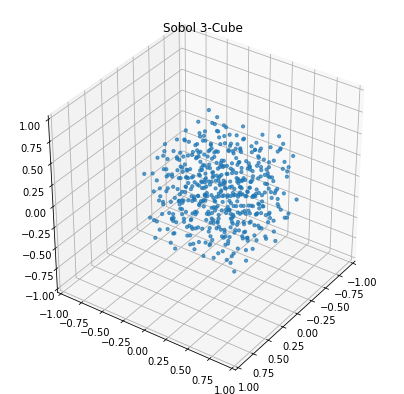
n_samples = 500
sample = Sobol().sample(n_samples, 3)
plot_3d(sample, 'Sobol 3-Cube')
plot_3d(normalize(sample - 0.5), 'Normalized Sobol 3-Cube')

/home/arvoelke/anaconda3/envs/py36/lib/python3.6/site-packages/ipykernel_launcher.py:14: RuntimeWarning: invalid value encountered in true_divide

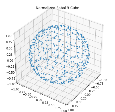
And it actually gets worse as the dimensionality goes up, because the volume of a \(D\)-cube is concentrated outside the region of the \(D\)-ball (and so vectors tend to get normalized to the corners)!

The following procedure (referred to as the “inverse transform method”) is a general way to sample an arbitrary multivariate random variable \({\bf X}\), using only the hyper-cube: 1. Pick a transformation \(T\) that maps each \({\bf x}\) to a vector \({\bf y} = T({\bf x})\) such that its components are mutually independent (might be identity). 2. Given the CDF of \({\bf X}\) and the chosen transformation, determine the CDF \(F\) of \({\bf Y}\) by a substitution of variables (hard part). 3. Then \({\bf x} = T^{-1}(F^{-1}({\bf z}))\) samples \({\bf X}\) uniformly, when \({\bf z}\) is sampled from a hyper-cube with the same dimensionality as \({\bf Y}\) (numerical part).

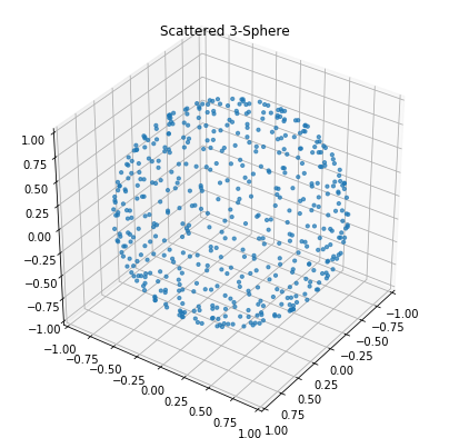
plot_3d(scatter_sphere.sample(n_samples, 3), 'Scattered 3-Sphere')

Spherical Coordinate Transformation

There’s a 10 page derivation in [1] for both the \(D\)-ball and \(D\)-sphere. The sphere case proceeds as follows: 1. The transformation \(T\) is the spherical coordinate transformation, such that \({\bf y}\) is a \((D-1)\)-dimensional vector of angles. 2. The distribution of the \(i^{th}\) element of \({\bf y}\) is:

\[\begin{split}F_i(y_i) = \begin{cases} \frac{1}{2} B(sin(\pi y_i)^2; \frac{D-i}{2}, \frac{1}{2}) & y_i < \frac{1}{2} \\ 1 - \frac{1}{2} B(sin(\pi y_i)^2; \frac{D-i}{2}, \frac{1}{2}) & otherwise \end{cases}, \quad i=1 \ldots D-1\end{split}\]

where \(B\) is the regularized incomplete beta function. 3. This distribution can be inverted using scipy’s betaincinv function. Also, \(T\) is easy to invert. Then take a scattered sample from the \((D-1)\)-cube and apply the inverse functions.

To modify this to work for the \(D\)-ball, we instead sample from the \(D\)-cube and take the last component to be a normalization coefficient for the resulting vector (by raising it to the power of \(\frac{1}{D}\)). See code for details.

Note: The distribution given by \(F\) is closely related to Jan’s SqrtBeta distribution of subvector lengths. They are identical after substituting the variable \(x = sin(\pi y_i)\) with \(n=1\) and \(m=D-i\), scaling by \(2\), and dealing with the reflection about \(y_i = \frac{1}{2}\).

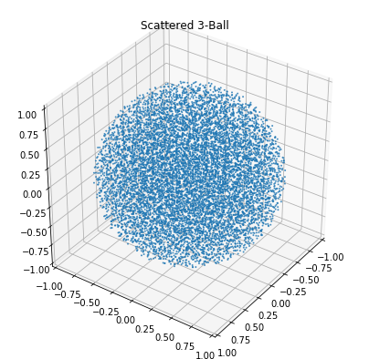
plot_3d(scatter_ball.sample(10000, 3), 'Scattered 3-Ball', 1)
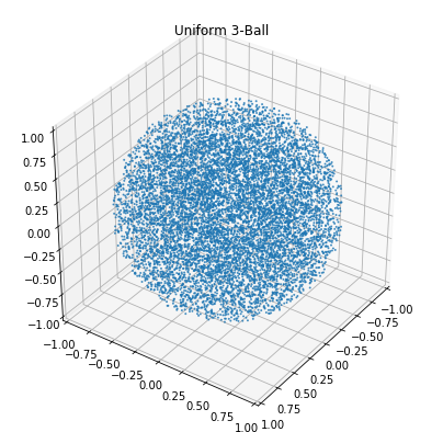
plot_3d(uniform_ball.sample(10000, 3), 'Uniform 3-Ball', 1)

Acknowledgements

Many thanks to Michael Hopkins from the SpiNNaker group in Manchester for providing me with all of the relevant background and reading material.

[1] K.-T. Fang and Y. Wang, Number-Theoretic Methods in Statistics. Chapman & Hall, 1994.