nengolib.signal.LinearSystem

signal.s = LinearSystem(sys=([1, 0], [1]), analog=True)

signal.z = LinearSystem(sys=([1, 0], [1]), analog=False)

class nengolib.signal.LinearSystem(sys, analog=None)

Generic linear system representation.

This extends nengo.LinearFilter to unify a variety of representations (transfer function, state-space, zero-pole gain) in continuous (i.e., analog) and discrete (i.e., digital) time-domains. Instances provide access to a number of common attributes and methods that are core to a variety of routines and networks throughout nengolib.

This can be used anywhere a nengo.synapses.Synapse (or nengo.LinearFilter) object is expected within Nengo. For instance, this can be passed as a synapse parameter to nengo.Connection. If the system is analog, then it will be automatically discretized using the simulation time-step (see cont2discrete()). We advocate for using this class to represent and manipulate linear systems whenever possible (e.g., to create synapse objects, and to specify dynamical systems, whenever modelling within the NEF).

The objects s and z are instances of LinearSystem that form the basic building blocks for analog or digital systems respectively (see examples). These objects respect the usual interpretation of differentiation and time-shifting in the Laplace– and z–domains respectively.

Parameters:

sys : linear_system_like

Linear system representation.

analog : boolean, optional

Continuous or discrete time-domain. Defaults to sys.analog if isinstance(sys, nengo.LinearFilter), otherwise True. If specified, it must not contradict sys.analog.

See also

s, z, LinearNetwork, ss2sim(), synapses

Notes

Instances of this class are intended to be immutable.

Currently, support is focused primarily on SISO systems. There is some limited support for SIMO, MISO, and MIMO systems within state-space representations, but the functionality of such systems is currently experimental / limited as they must remain in state-space form.

State-space representations must be causal (proper) and finite. Transfer functions must also be finite (Padé approximants may help here) but may be acausal (not necessarily proper) and must remain SISO.

Conversions between representations are cached within the object itself. Redundantly casting a LinearSystem to itself returns the same underlying object, in order to persist this cache whenever possible. This is done not as a performance measure, but to guard against numerical issues that would result from accidentally converting back and forth between the same formats.

Examples

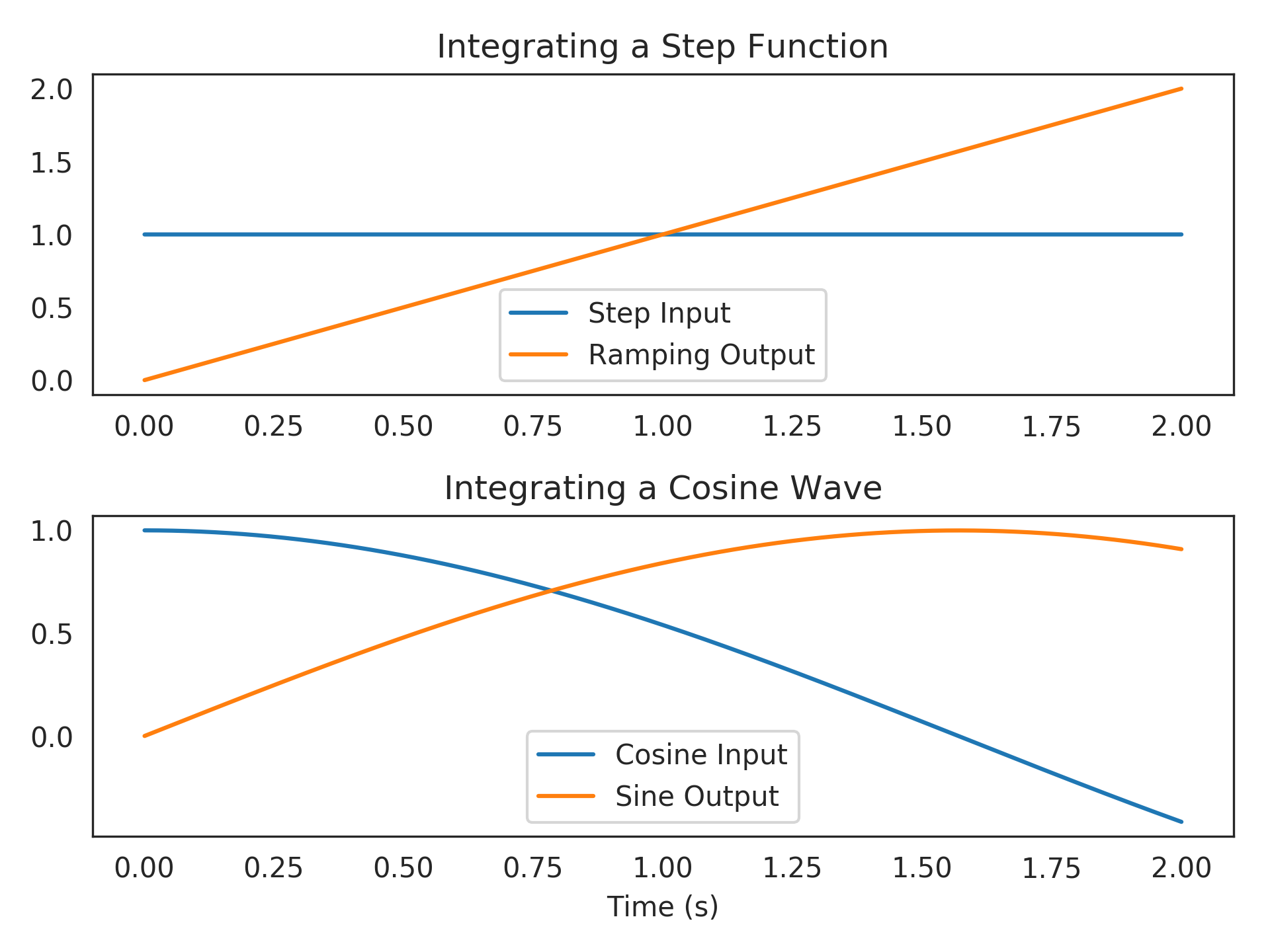
A simple continuous-time integrator:

>>> from nengolib.signal import s
>>> integrator = 1/s
>>> assert integrator == ~s == s**(-1)
>>> t = integrator.trange(2.)
>>> step = np.ones_like(t)
>>> cosine = np.cos(t)

>>> import matplotlib.pyplot as plt
>>> plt.subplot(211)
>>> plt.title("Integrating a Step Function")
>>> plt.plot(t, step, label="Step Input")
>>> plt.plot(t, integrator.filt(step), label="Ramping Output")
>>> plt.legend(loc='lower center')
>>> plt.subplot(212)
>>> plt.title("Integrating a Cosine Wave")
>>> plt.plot(t, cosine, label="Cosine Input")
>>> plt.plot(t, integrator.filt(cosine), label="Sine Output")
>>> plt.xlabel("Time (s)")
>>> plt.legend(loc='lower center')
>>> plt.show()

(Source code)

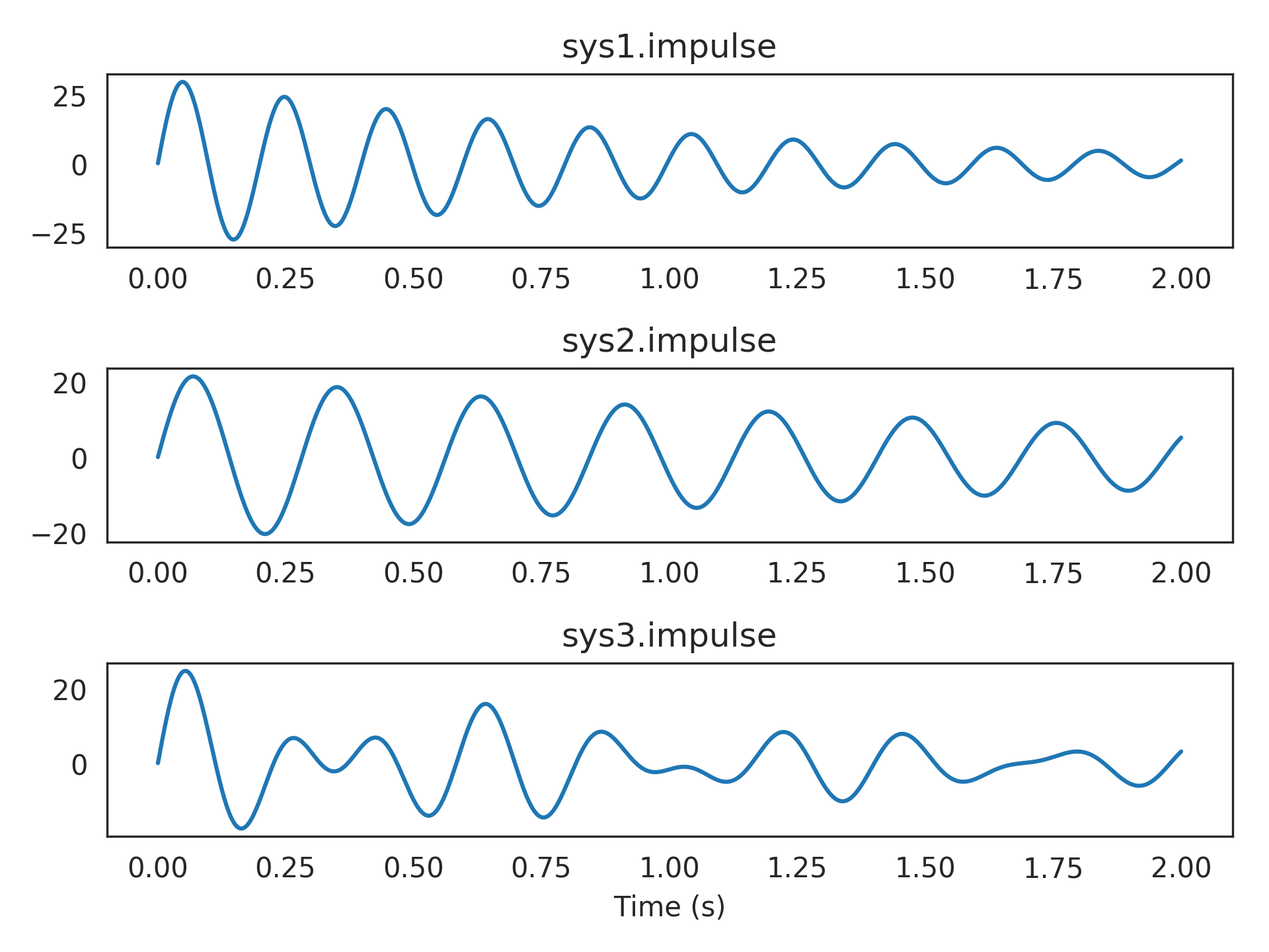
Building up higher-order continuous systems:

>>> sys1 = 1000/(s**2 + 2*s + 1000)   # Bandpass filtering
>>> sys2 = 500/(s**2 + s + 500)       # Bandpass filtering
>>> sys3 = .5*sys1 + .5*sys2          # Mixture of two bandpass
>>> assert len(sys1) == 2  # sys1.order_den
>>> assert len(sys2) == 2  # sys2.order_den
>>> assert len(sys3) == 4  # sys3.order_den

>>> plt.subplot(311)
>>> plt.title("sys1.impulse")
>>> plt.plot(t, sys1.impulse(len(t)), label="sys1")
>>> plt.subplot(312)
>>> plt.title("sys2.impulse")
>>> plt.plot(t, sys2.impulse(len(t)), label="sys2")
>>> plt.subplot(313)
>>> plt.title("sys3.impulse")
>>> plt.plot(t, sys3.impulse(len(t)), label="sys3")
>>> plt.xlabel("Time (s)")
>>> plt.show()

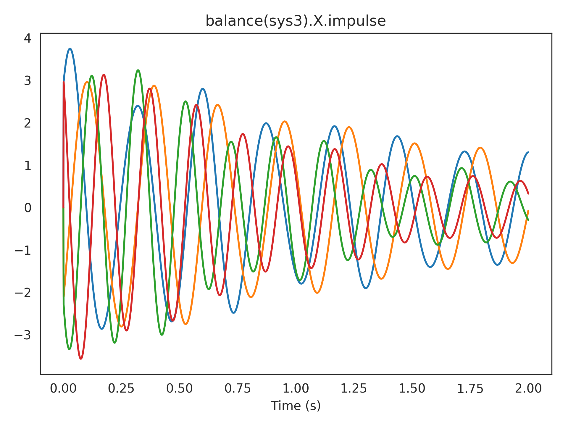
Plotting a linear transformation of the state-space from sys3.impulse:

>>> from nengolib.signal import balance
>>> plt.title("balance(sys3).X.impulse")
>>> plt.plot(t, balance(sys3).X.impulse(len(t)))
>>> plt.xlabel("Time (s)")
>>> plt.show()

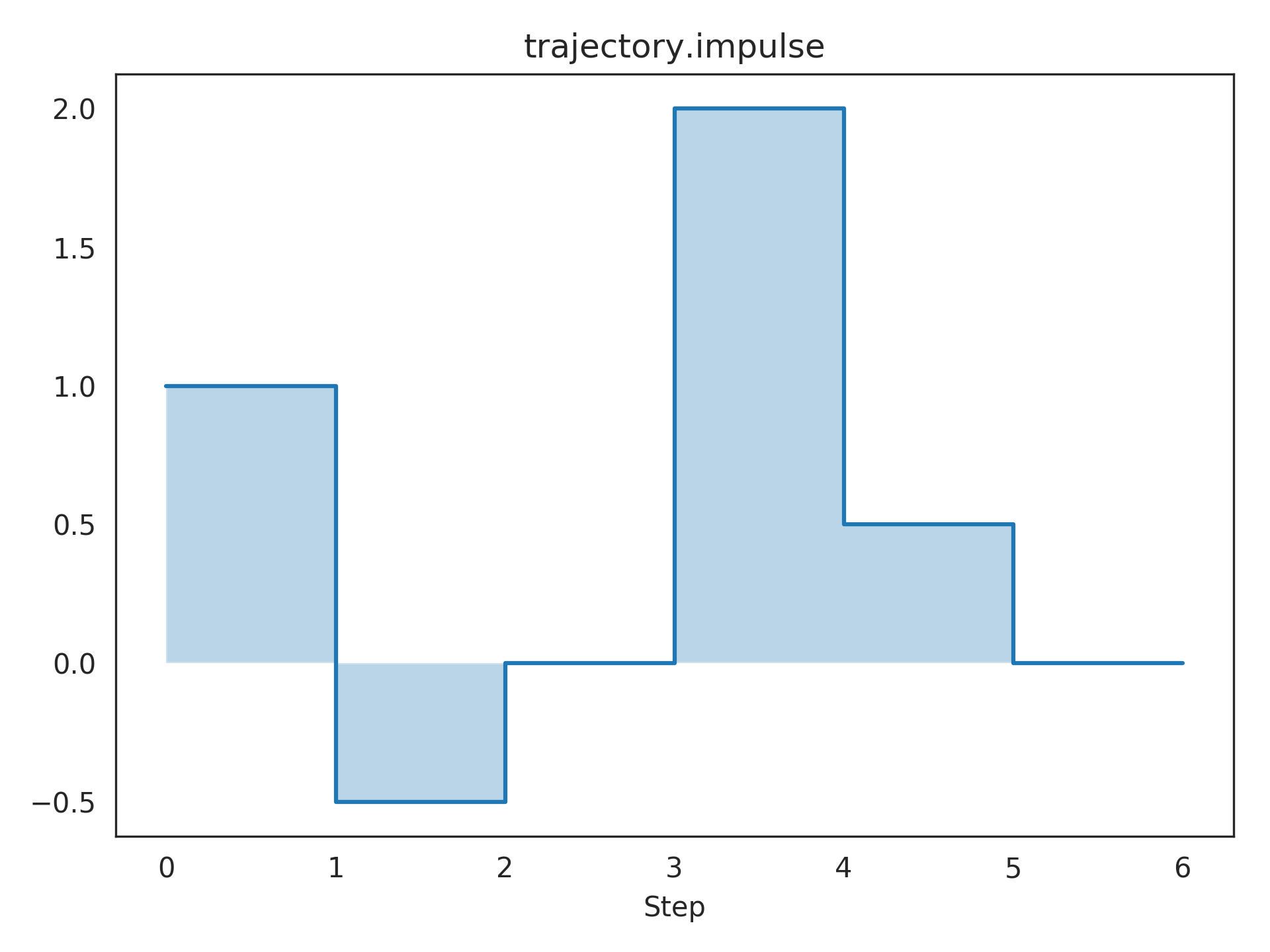
A discrete trajectory:

>>> from nengolib.signal import z
>>> trajectory = 1 - .5/z + 2/z**3 + .5/z**4
>>> t = np.arange(7)
>>> y = trajectory.impulse(len(t))

>>> plt.title("trajectory.impulse")
>>> plt.step(t, y, where='post')
>>> plt.fill_between(t, np.zeros_like(y), y, step='post', alpha=.3)
>>> plt.xticks(t)
>>> plt.xlabel("Step")
>>> plt.show()

Attributes:

A

A matrix from state-space representation.

B

B matrix from state-space representation.

C

C matrix from state-space representation.

D

D matrix from state-space representation.

X

Returns the multiple-output system for the state-space vector.

analog

Boolean indicating whether system is analog or digital.

causal

Boolean indicating if the system is causal / proper.

controllable

Returns a new system in controllable canonical form.

dcgain

Steady-state response to unit step input.

default_size_in

A parameter where the value is an integer.

default_size_out

A parameter where the value is an integer.

den

Denominator of transfer function.

gain

Gain from zero-pole gain representation.

has_passthrough

Boolean indicating if the system has a passthrough.

is_SISO

Boolean indicating whether system is SISO.

is_ss

Boolean indicating whether state-space has been computed.

is_stable

Boolean indicating if system is exponentially stable.

is_tf

Boolean indicating whether transfer function has been computed.

is_zpk

Boolean indicating whether zero-pole gain has been computed.

num

Numerator of transfer function.

observable

Returns a new system in observable canonical form.

order_den

Order of transfer function’s denominator (i.e., state dimension).

order_num

Order of transfer function’s numerator.

poles

Poles from zero-pole gain representation.

seed

shape

Short-hand for (.size_in, .size_out).

size_in

Input dimensionality (this equals 1 for SISO or SIMO).

size_out

Output dimensionality (this equals 1 for SISO or MISO).

ss

State-space representation (A, B, C, D).

strictly_proper

Boolean indicating if the system is strictly proper.

tf

Transfer function representation (num, den).

zeros

Zeros from zero-pole gain representation.

zpk

Zero-pole gain representation (zeros, poles, gain).

Methods

General(num, den, output[, y0])	An LTI step function for any given transfer function.
NoDen(num, den, output)	An LTI step function for transfer functions with no denominator.
Simple(num, den, output[, y0])	An LTI step function for transfer functions with one num and den.
Step(num, den, output)	Abstract base class for LTI filtering step functions.
__call__(s)	Evaluate the transfer function at the given complex value(s).
apply(x[, d, dt, rng, copy])	Run process on a given input.
combine(obj)	Combine in series with another LinearFilter.
evaluate(frequencies)	Evaluate the transfer function at the given frequencies.
filt(u[, dt, axis, y0, copy, filtfilt])	Filter the input using this linear system.
filtfilt(x, **kwargs)	Zero-phase filtering of x using this filter.
get_rng(rng)	Get a properly seeded independent RNG for the process step.
impulse(length[, dt])	Impulse response with length timesteps and width dt.
make_step(shape_in, shape_out, dt, rng[, …])	Produces the function for filtering across one time-step.
ntrange(n_steps[, dt])	Create time points corresponding to a given number of steps.
run(t[, d, dt, rng])	Run process without input for given length of time.
run_steps(n_steps[, d, dt, rng])	Run process without input for given number of steps.
trange(t[, dt])	Create time points corresponding to a given length of time.
transform(T[, Tinv])	Changes basis of state-space matrices to T.

Subset of magic methods

__len__()	Dimensionality of state vector.
__invert__()	Reciprocal of transfer function.
__neg__()
__pow__(other)
__add__(other)
__sub__(other)
__mul__(other)
__div__(other)
__eq__(other)