nengolib.stats.spherical_transform

nengolib.stats.spherical_transform(samples)

Map samples from the [0, 1]–cube onto the hypersphere.

Applies the inverse transform method to the distribution SphericalCoords to map uniform samples from the [0, 1]–cube onto the surface of the hypersphere. [1]

Parameters:

samples : (n, d) array_like

n uniform samples from the d-dimensional [0, 1]–cube.

Returns:

mapped_samples : (n, d+1) np.array

n uniform samples from the d–dimensional sphere (Euclidean dimension of d+1).

See also

Rd, Sobol, ScatteredHypersphere, SphericalCoords

References

[1]	K.-T. Fang and Y. Wang, Number-Theoretic Methods in Statistics. Chapman & Hall, 1994.

Examples

>>> from nengolib.stats import spherical_transform

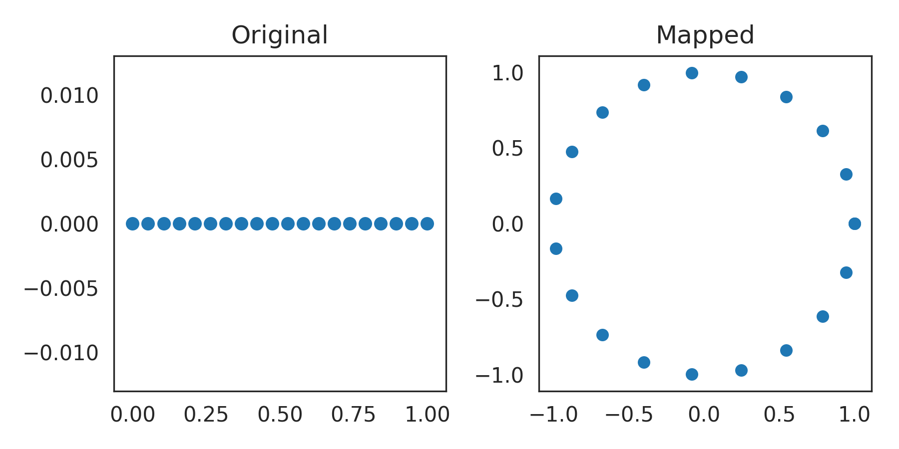
In the simplest case, we can map a one-dimensional uniform distribution onto a circle:

>>> line = np.linspace(0, 1, 20)
>>> mapped = spherical_transform(line)

>>> import matplotlib.pyplot as plt
>>> plt.figure(figsize=(6, 3))
>>> plt.subplot(121)
>>> plt.title("Original")
>>> plt.scatter(line, np.zeros_like(line), s=30)
>>> plt.subplot(122)
>>> plt.title("Mapped")
>>> plt.scatter(*mapped.T, s=25)
>>> plt.show()

(Source code)

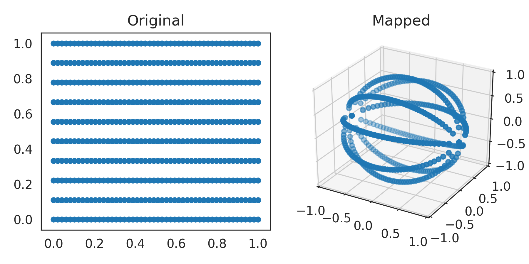
This technique also generalizes to less trivial situations, for instance mapping a square onto a sphere:

>>> square = np.asarray([[x, y] for x in np.linspace(0, 1, 50)
>>>                             for y in np.linspace(0, 1, 10)])
>>> mapped = spherical_transform(square)

>>> from mpl_toolkits.mplot3d import Axes3D
>>> plt.figure(figsize=(6, 3))
>>> plt.subplot(121)
>>> plt.title("Original")
>>> plt.scatter(*square.T, s=15)
>>> ax = plt.subplot(122, projection='3d')
>>> ax.set_title("Mapped").set_y(1.)
>>> ax.patch.set_facecolor('white')
>>> ax.set_xlim3d(-1, 1)
>>> ax.set_ylim3d(-1, 1)
>>> ax.set_zlim3d(-1, 1)
>>> ax.scatter(*mapped.T, s=15)
>>> plt.show()