nengolib.synapses.Bandpass

nengolib.synapses.Bandpass(freq, Q)

A second-order bandpass with given frequency and width.

Parameters:

freq : float

Frequency (in hertz) of the peak of the bandpass.

Q : float

Inversely proportional to width of bandpass.

Returns:

sys : LinearSystem

Second-order lowpass with complex poles.

See also

nengo.networks.Oscillator()

Notes

The state of this system is isomorphic to a decaying 2–dimensional oscillator with speed given by freq and decay given by Q.

References

[1]	http://www.analog.com/library/analogDialogue/archives/43-09/EDCh%208%20filter.pdf

Examples

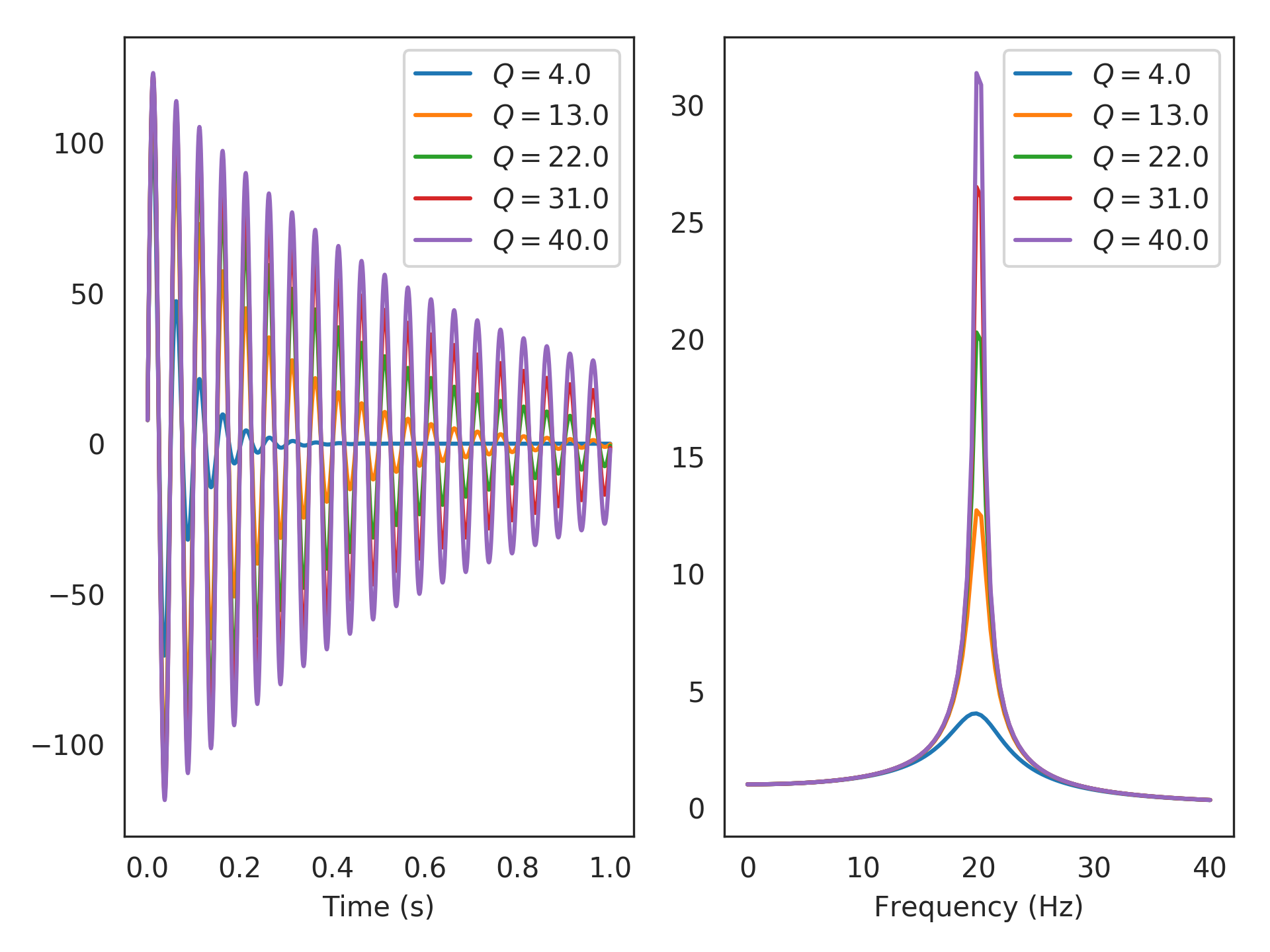
Bandpass filters centered around 20 Hz with varying bandwidths:

>>> from nengolib.synapses import Bandpass
>>> freq = 20
>>> Qs = np.linspace(4, 40, 5)

Evaluate each impulse (time-domain) response:

>>> import matplotlib.pyplot as plt
>>> plt.subplot(121)
>>> for Q in Qs:
>>>     sys = Bandpass(freq, Q)
>>>     plt.plot(sys.ntrange(1000), sys.impulse(1000),
>>>              label=r"$Q=%s$" % Q)
>>> plt.xlabel("Time (s)")
>>> plt.legend()

Evaluate each frequency responses:

>>> plt.subplot(122)
>>> freqs = np.linspace(0, 40, 100)  # to evaluate
>>> for Q in Qs:
>>>     sys = Bandpass(freq, Q)
>>>     plt.plot(freqs, np.abs(sys.evaluate(freqs)),
>>>              label=r"$Q=%s$" % Q)
>>> plt.xlabel("Frequency (Hz)")
>>> plt.legend()
>>> plt.show()

(Source code)

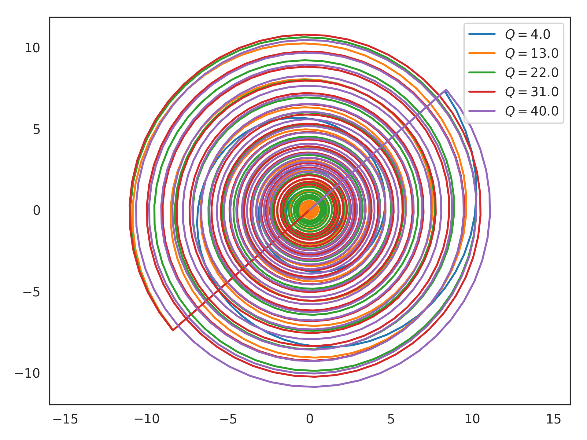
Evaluate each state-space impulse (trajectory) after balancing:

>>> from nengolib.signal import balance
>>> for Q in Qs:
>>>     plt.plot(*balance(Bandpass(freq, Q)).X.impulse(1000).T,
>>>              label=r"$Q=%s$" % Q)
>>> plt.legend()
>>> plt.axis('equal')
>>> plt.show()