nengolib.synapses.PadeDelay

nengolib.synapses.PadeDelay(theta, order, p=None)

A finite-order approximation of a pure time-delay.

Implements the transfer function:

\[F(s) = e^{-\theta s} + \mathcal{O}(s^{\texttt{order}+\texttt{p}})\]

or \(y(t) \approx u(t - \theta)\) in the time-domain (for slowly changing inputs).

This is the optimal approximation for a time-delay system given low-frequency inputs implemented using a finite-dimensional state. This is achieved via Padé approximants. The state-space of the system encodes a rolling window of input history (see RollingWindow). This can be used to approximate FIR filters and window functions in continuous time.

Parameters:

theta : float

Length of time-delay in seconds.

order : integer

Order of approximation in the denominator (dimensionality of resulting system).

p : integer, optional

Order of approximation in the numerator. Defaults to p=order-1, since this gives the highest-order approximation without a passthrough. If p=order, then the system will have a passthrough, which has a nonideal step response.

Returns:

sys : LinearSystem

Finite-order approximation of a pure time-delay.

See also

LegendreDelay(), pade_delay_error(), RollingWindow, DiscreteDelay(), scipy.misc.pade()

Notes

Closed-form derivations are found in [1].

References

[1]	A. R. Voelker and C. Eliasmith, “Improving spiking dynamical networks: Accurate delays, higher-order synapses, and time cells”, 2017, Submitted. [URL]

Examples

>>> from nengolib.synapses import PadeDelay

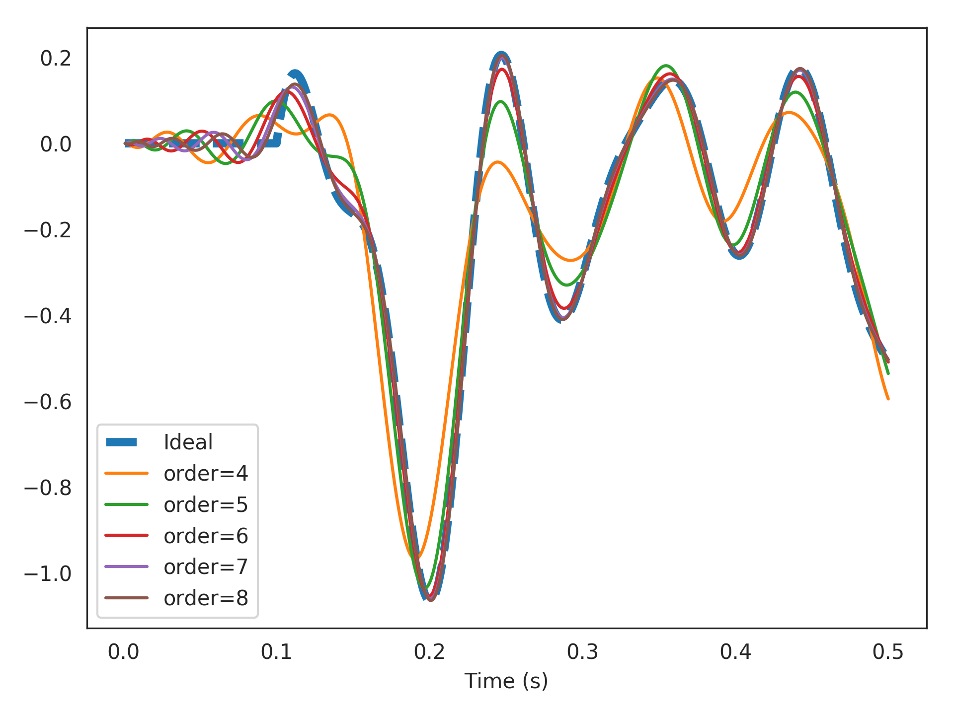
Delay 15 Hz band-limited white noise by 100 ms using various orders of approximations:

>>> from nengolib.signal import z
>>> from nengo.processes import WhiteSignal
>>> import matplotlib.pyplot as plt
>>> process = WhiteSignal(10., high=15, y0=0)
>>> u = process.run_steps(500)
>>> t = process.ntrange(len(u))
>>> plt.plot(t, (z**-100).filt(u), linestyle='--', lw=4, label="Ideal")
>>> for order in list(range(4, 9)):
>>>     sys = PadeDelay(.1, order=order)
>>>     assert len(sys) == order
>>>     plt.plot(t, sys.filt(u), label="order=%s" % order)
>>> plt.xlabel("Time (s)")
>>> plt.legend()
>>> plt.show()

(Source code)

nengolib.synapses.pade_delay_error

nengolib.synapses.pade_delay_error(theta_times_freq, order, p=None)

Computes the approximation error in PadeDelay().

For a given order, the difficulty of the delay is a function of the input frequency (\(s = 2j \pi f\)) times the delay length (\(\theta\)).

Parameters:

theta_times_freq : array_like

A float or array of floats (delay length times frequency) at which to evaluate the error.

order : integer

order parameter passed to PadeDelay().

p : integer, optional

p parameter passed to PadeDelay(). Defaults to None.

Returns:

error : np.array of np.complex

Shaped like theta_times_freq, with each element corresponding to the complex error term

\[F(2j \pi f) - e^{-\theta \times 2j \pi f}\]

where \(F(s)\) is the transfer function constructed by PadeDelay() for a delay of length \(\theta\).

See also

PadeDelay()

Examples

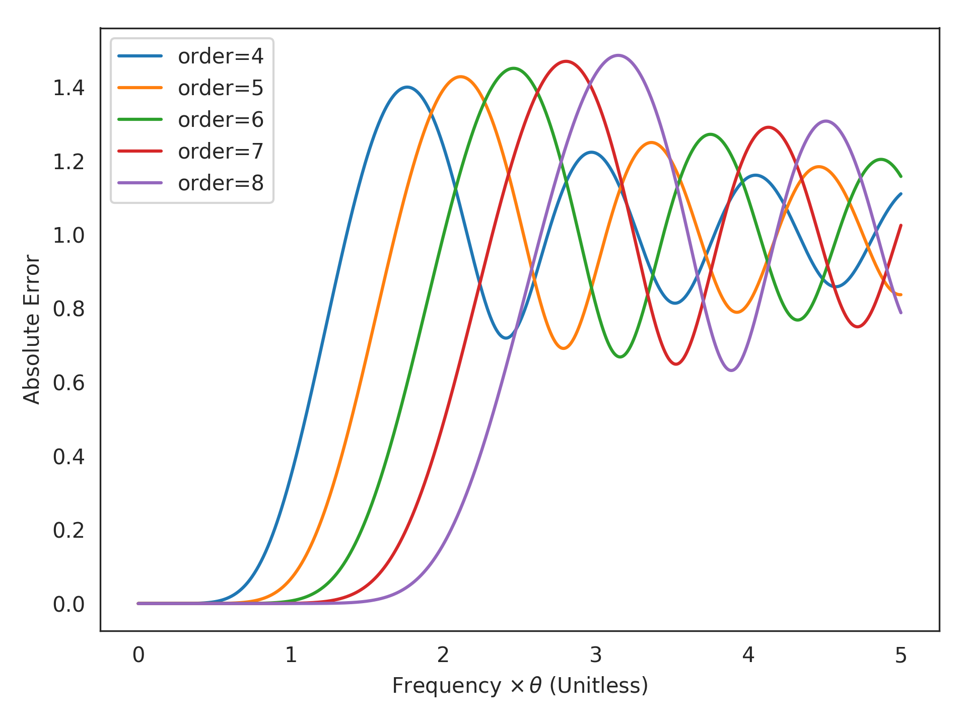
>>> from nengolib.synapses import pade_delay_error
>>> abs(pade_delay_error(1, order=6))
0.0070350205992081461

This means that for order=6 and frequencies less than 1/theta, the approximation error is less than one percent!

Now visualize the error across a range of frequencies, with various orders:

>>> import matplotlib.pyplot as plt
>>> freq_times_theta = np.linspace(0, 5, 1000)
>>> for order in range(4, 9):
>>>     plt.plot(freq_times_theta,
>>>              abs(pade_delay_error(freq_times_theta, order=order)),
>>>              label="order=%s" % order)
>>> plt.xlabel(r"Frequency $\times \, \theta$ (Unitless)")
>>> plt.ylabel("Absolute Error")
>>> plt.legend()
>>> plt.show()

(Source code)